Curves are clustered with the CCToolbox by following five simple steps.
You must run SetCCTPath() each time you wish to use the toolbox. This function sets the appropriate paths needed by the toolbox. You can run this each time automatically by starting matlab with the -r option.
Curves can be represented in various ways (see curve formats for more details). The standard way that they are represented in the toolbox is by loading a set of curves into cell arrays. For example, suppose we have n curves, then the observations for each of these curves are stored in the n-by-1 cell array Y. The times (or whichever independent variable is of interest) at which these observations were made is stored in the cell array X of the same size. Thus, the i-th curve's observations Y{i} and observation times X{i} can be easily accessed using the index variable i.
Since observations can be multivariate (say, of dimension D) and curve lengths may vary (say, length ni for curve i), the size of each Y{i} is ni by D, where the total number of observations in all curves is N=n1+n2+...+nn. The size of each X{i} is always ni by 1 since time is univariate. However, often the times at which the curve observations were made are fixed and uniform across all curves. In this case, X does not actually have to be specified, and the toolbox assumes that X{i} is equal to 0..(ni -1).
As an example, we demonstrate the structure of a set of curves representing actual observed cyclone tracks that originated in the North Atlantic from 1995-2001. Each track consists of ni observations of cyclone latitude and longitude position, and there are 296 total tracks. The size of the cell array Y as output by Matlab can be seen below.
 >> whos Y
  Name      Size                   Bytes  Class

  Y       296x1                    87152  cell array
The cells for the first 10 tracks can be listed as follows.
 >> Y(1:10)
ans =
    [13x2 double]
    [10x2 double]
    [21x2 double]
    [11x2 double]
    [18x2 double]
    [14x2 double]
    [14x2 double]
    [10x2 double]
    [10x2 double]
    [19x2 double]
Notice that, for example, the first track Y{1} has 13 observations, each being two-dimensional (i.e., both a latitude and longitude observation). The first track can be listed as follows.
 >> Y{1}
ans =
  -57.2177   51.2200
  -55.5783   53.1028
  -54.8666   55.2942
  -55.0624   57.3329
  -56.4487   58.9460
  -57.2662   59.2198
  -57.9229   59.5291
  -57.8100   59.3403
  -57.1867   59.6936
  -57.5489   60.9830
  -55.9977   61.8928
  -62.3653   65.1744
  -62.8327   67.4031
The first dimension here is longitude and the second is latitude, although this ordering is insignificant. (Negative longitude numbers mean west of zero degrees and positive latitude numbers mean north of zero degrees.) A plot of the first 10 cyclone tracks on a map of the North Atlantic is given below. The small circles indicate the genesis point (the origin) for each cyclone track.
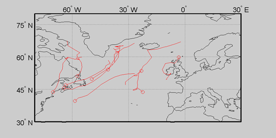
For this data set there is no need for an X cell array since each cyclone track was observed uniformly at 6-hour intervals from time zero (the instant at which it was detected) to time ni (the end of its lifetime). In the absence of a provided X cell array, the toolbox simply assumes that X{i} is equal to 0..(ni -1).
Depending on the particular cluster model that is used (see cluster models for complete list), there are a number of different model options. For example, knots are required for spline regression but not for polynomial regression. In any case, all options are set by using one large options structure.
You can retrieve the default options for any cluster model by calling the clustering function associated with that model and passing-in the single string argument of 'options'. For example, ops = lrm('options') will return the default options for linear/polynomial regression mixtures in ops.
Most cluster models only require the most common options. These are listed below.
| ops.method | : select clustering method; see listmodels() for all methods | |
| ops.K | : number of clusters | |
| ops.order | : order of regression; specify 1 for linear, 2 for quadratic, etc. | |
| ops.zero | : select data normalization; see trajs2seq() for values |
The help message at the beginning of each clustering function should list any other required options for that model. For example, ops.knots is required for srm(); however, even in this case it is possible to enable automatic knot selection, and thus dispense with specifying ops.knots.
For our current demo using the cyclone track data, we set only the basic options as follows.
ops =
    method: 'lrm'
         K: 3
     order: 2
      zero: 'none'
We are going to use standard linear/polynomial regression mixtures as specified by 'lrm', and we are seeking three groups in the data. We choose to use quadratic polynomial regression, and we do not want to perform any preprocessing or normalization of the data.
Unlike the cluster model options, the EM options of this section are all truly optional. These options are more technical in nature and usually apply to all EM algorithms in general, regardless of the cluster model. Some of the more common options are listed below.
| ops.NumEMStarts | : number of random EM starts to perform | |
| ops.IterLimit | : maximum number of possible iterations to perform | |
| ops.stopval | : value used in EM stopping criterion function (e.g., see lrm()) | |
| ops.ShowGraphics | : {0,1} enable iterative graphics output during EM |
For our current demo, we only set the number of random EM starts.
>> ops.NumEMStarts = 5;
The clustering is carried out by calling curve_clust() and passing-in the curve data and the options structure.
>> model = curve_clust(Y,ops);
When the clustering is finished, a learned model structure is returned. The format of this structure is detailed extensively in the model structure section of the documentation. For the sake of completeness, we list this structure here.
>> model
model =
                 K: 3
             order: 2
           Options: [1x1 struct]
              zero: 'none'
            method: 'lrm'
               Pik: [296x3 double]
             Alpha: [3x1 double]
                Mu: [3x3x2 double]
             Sigma: [2x2x3 double]
             scale: 5.3632e-004
             Lhood: [1x30 double]
                 C: [296x1 double]
         NumPoints: 8674
        TrainLhood: -3.0850e+004
    TrainLhood_ppt: -3.5565
      NumIndParams: 26
             state: [35x1 double]
            nstate: [2x1 double]
Of the five random EM starts, the one with maximum likelihood is always returned. This maximal run consisted of 30 iterations as can be seen by the size of model.Lhood, which gives the log-likelihood achieved at each iteration of EM. The final log-likelihood value is -3.0850e+004 (as given by model.TrainLhood) and the final per-point log-likelihood value is -3.5565 as shown by model.TrainLhood_ppt.
The regression coefficients are stored in model.Mu. For example, model.Mu(:,1,1) holds the longitudinal coefficients for cluster one, while model.Mu(:,2,1) holds them for cluster two. Finishing up, we note that the actual clustering is given by reading the labels stored in model.C. For example, the labels for the first ten tracks are as shown below.
>> model.C(1:10)
ans =
     2
     1
     1
     1
     3
     1
     1
     1
     1
     2
You can visualize the results of the clustering by calling showmodel().
>> showmodel(model,Y);
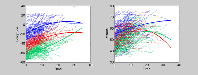
The left plot shows the longitude vs. time profiles for all of the tracks, and the right plot shows the latitude vs. time profiles. The learned cluster groups are color-coded, and the mean curves for each group are bolded. There are many options that can be used to change the type of plot produced with showmodel(). The function is set up like a large script with all of the options laid out and explained, line-by-line. The user is encouraged to actively edit and re-edit this function/script to produce the desired plots.
Since this data is inherently geographic, it can be effective to view the clustering on top of the map from whence the data originated. This type of plot can be produced with the Cyclone Tracking Toolbox.
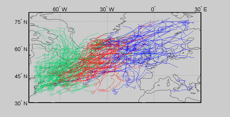
Notice that the clusters appear to be heavily influenced by initial cyclone track position (or genesis position). This can be seen as a benefit or a nuisance. One can remove this dependence by using advanced options. This will be briefly discussed in the next section.
In the previous exercise, we used standard polynomial regression mixtures to perform the clustering. We might like to try other methods that allow for continuous alignment in time, such as lrm_b() (see cluster models for a complete list of models). This will allow for two cyclone tracks that are similar but translated in time to be simultaneously aligned and clustered. This clustering method can be tried by simply changing the value of ops.method as follows.
>> ops.method = 'lrm_b';
That's it. Now you can just run curve_clust() directly as before.
Suppose we now would like to remove initial starting position as a possible source of variation. We can easily do this by changing the value of ops.zero. One setting for this option is the string 'zero'. This will take each cyclone track and subtract the first lat-lon position from each of the measurements for that cyclone. This will force all cyclones to begin at the relative position of (0,0), and hence remove initial starting position as a possible source of variation.
>> ops.zero = 'zero'
ops =
         method: 'lrm'
              K: 3
          order: 2
           zero: 'zero'
    NumEMStarts: 5
Now we simply run the clustering and plot the results again.
>> model_zero = curve_clust(Y,ops);
>> showmodel(model_zero,Y);

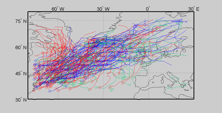
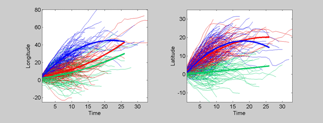
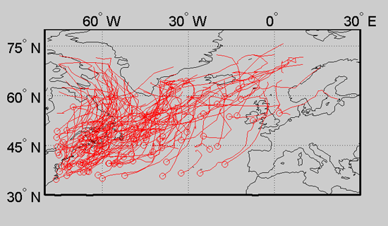
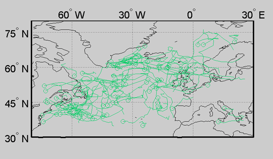
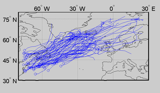
Now we have clearly removed initial starting position as a source of variation. The clustering is more concentrated on cyclone track shape as a result. This can better be seen in the following three cluster plots.
This concludes the tutorial. More information can be found on the main documentation page.